PROJECT MANAGEMENT
Self-contained mini-workspaces, where sample sets can be analyzed independently without interference from other data, using multiple pipelines.
- SAMPLE SET MANAGEMENT
- Project Setup
- Pipeline Management
- Favorites Pipelines
- My Pipelines
- Pipeline Creation
- Pipeline Filters
- Copy Pipeline
- De Novo Pipeline
- Pipeline Execution
- Reports
- Jobs
SAMPLE SET MANAGEMENT
Sample Set is a group of sequence files that belong to an experiment and can be analyzed together. Sample Set window allows new sample set creation and provides a list view of the existing Sample Sets within a project (Fig. 1).

Sample Set Creation
Sample Set can be created by selecting the samples available in the. Click from the Project Main window or click on the Sample Set window to create a new Sample Set (Fig. 2).

Fill in the following details on the Sample Set creation window:
-
- Name* - Provide a unique name for the Sample Set.
Only alphanumeric characters and spaces are allowed.
Sample Set names are helpful while executing the pipelines.
CAUTION - Names shouldn’t be reused.
-
- Description* - Provide a description for the Sample Set that can be included in the final report (Example: experiment type).
- Organism - Select organism name from the drop-down list.
Samples from different organisms can be selected to form a single sample set
CAUTION - Unless intended, samples from multiple organisms in a sample set are not recommended.
-
- Select Tag - Using the tags given during sample upload samples can be filtered. A list of samples uploaded under the corresponding tag would appear in the table on the left. Click on the samples to move them to the selected samples table and to add to the sample set (Fig. 2). icon allows moving all the samples listed under the selected tag to the selected samples table.icons allow deselection of the selected samples (Fig. 2).
Samples from different tags can be selected to create one sample set.
CAUTION - Select either SE or PE samples only. The platform doesn’t allow mixed selection.
Sample Filter
Click on the to filter samples based on the sample quality. Six filters are supported.
-
-
-
-
- The total number of reads: This shows the samples with the total number of reads greater than the number entered.
- Number of poor quality reads: This shows the samples which contain, number of poor quality reads less than the number entered. The quality of reads is determined by the fastqc tool.
- Sequence length: Shows the samples with reads whose sequence length ranges the number entered.
- Per base sequence quality: Shows the samples with reads per base sequence quality tagged as Pass/Fail/Warn.
- Sequence length distribution: This shows the samples with reads sequence length distribution tagged as Pass/Fail/Warn.
- Adapter content: Shows the samples with read adapter content tagged as Pass/Fail/Warn.
-
-
-
Click on the upper right corner of the window to save the Sample Set. Multiple sample sets can be created under one project with different sequence files.
Sample Set Deletion
A sample set can be deleted by clicking icon on the Sample Set window. This action deletes the sample set only, however, the samples are still available in the Sequence Data for future usage.
Project Setup
A new project can be created in two ways.
- From the Dashboard window - click the icon
- From the Projects window - click on the upper right corner

A new project can be created from the Project setup window (Fig. 1). Fill in the seven mandatory fields with details and appropriate descriptions. The data in this form is used for automatic reference file(s) selection and will be exported to the final report.
CAUTION - Organism enables appropriate reference file(s) selection.
-
- Name* - Provide a unique name for the project.
HINT - Project name cannot be longer than 30 characters and alphanumeric characters and spaces are only allowed.
CAUTION - Project name should be unique.
-
- Organism* - Select the organism from the drop-down menu. We currently support eight main model organisms and some custom species.
HINT - Select Other if the organism is not listed and contact Stanome technical support team to add a new organism to the list.
-
- Description* - Provide a brief description of the project (Example: The gist of the experimental design and the aim of the study).
- Data Type* - Select sample type from the drop-down list [Microbiome, Targeted Genome, Transcriptome, and Whole Genome]. The Data type field is tightly connected with the Hub field in the pipelines.
HINT - Carefully choose the Data type to get the relevant pipeline suggestions.
-
- Analysis Type* - Select the experiment type from the drop-down list [ABR Screening, Alignment, Annotations, Data Cleaning, Data QC, Differential Expression, Genome assembly, Genotyping, Proband, Serotyping, Species Classification, and Variant analysis].
- Expected output* - Select expected output(s) from the drop-down list [BAM, Coverage Metrics, DE Genes (Differentially Expressed Gene list), FASTA, Genotypes, Ontology, Pathways, and VCF (Variant Calling Format)].
Multiple options can be selected.
-
- Details* - Provide detailed information about the project. (Example: Aim of the experiment, conditions studied, experimental design, and any other pertinent details).
Click to save the project. The new project is saved and displays the Project Main window (Fig. 2), where the project-specific menu is available on the left menu. The project can be navigated with Sample Set, My Pipelines, Jobs, and Reports, and details of these four features are described in the following sections.

Projects can be deleted using the icon from the Projects window. All the components within a project (sample sets, pipelines, jobs, and reports) are deleted permanently.
Pipeline Management
A set of computational tools, which run either sequentially or parallelly in order to achieve a specific data analysis objective. Tools/commands are designated as steps in a pipeline.
Favorites Pipelines
Pipelines, from any project, can be added or deleted from the favorites by clicking the icon next to the pipeline name in the list view i.e. My Pipelines. Stanome owned pipelines can’t be added to the favorites. Favorite pipelines are visible in the Pipeline Library and My Pipelines (filtered based on the Owner, Hub, and Category).
My Pipelines
My Pipelines show the list of pipelines within a project. Pipelines can be created, viewed, edited, and deleted within the project scope. My Pipelines is empty, by default, and users can create new pipelines de novo or copy the pre-configured pipelines from the Pipeline Library. Follow the instructions in the next section to create a pipeline.
Pipeline Creation
The new pipeline creation window is accessed from two locations. Either click on the project window or click on the My Pipelines window to create a new pipeline (Fig. 1).

The new pipeline creation window displays three icons in the upper right corner.
Exit out of the pipeline creation without saving.
Save the pipeline.
Copy pipeline.
New pipelines can be added to a project in three ways.
- Copying pre-configured pipelines
- Creating de novo
- Favorite pipeline
Pipeline Filters
Pipelines on the platform are tightly connected with the projects. The Data type field in the projects is tied with the Hub field in the pipelines. Based on the Data Type definition in the project setup, only relevant pipelines are shown. The following table shows the corresponding terms between projects and pipelines.
|
Data Type in Project |
Pipeline Hub |
|
Whole Genome |
Genome |
|
Microbiome |
Micro |
|
Transcriptome |
Transcript |
|
Targeted Genome |
Variant |
Table 4: Terms associated between projects and pipelines
Copy Pipeline
A new pipeline can be created by copying an existing pipeline from other projects or a pre-configured pipeline from Pipeline Library.
Click in the upper right corner of the pipeline creation window to see the existing pipelines via the Select pipeline dialog box (Fig.). Using the project setup information, a list of prefiltered pipelines is listed. Users can use multiple field combinations to filter the pipelines. Pipelines from the can be viewed by selecting the owner as “Stanome”. Select a pipeline and click on to copy a pipeline into the current project. The pipeline steps, tools, parameters, and other details are auto-populated (except the pipeline name). Name the new pipeline uniquely (duplicate names are not allowed) and verify the tools and commands before saving the pipeline.
HINT: Pipeline name should be less than 50 characters long and only alphanumeric characters and spaces are allowed.

De Novo Pipeline
De novo pipeline building requires bioinformatics expertise. Please contact the technical support team for assistance.
The creation of a brand new pipeline is more challenging than copying an existing pipeline. Fill in the following details on the pipeline creation window (Fig. 1) to create a new pipeline. Mandatory fields are indicated with asterisks (*).
- Name* - Provide a unique name
- Execution Flow* - Enter the tool names in the order of execution (e.g. Trimmomatic -> Salmon -> Sleuth)
- Hub* - Indicate the pipeline group
- Category* - Select the functional category
- Description* - Provide a brief description of the pipeline’s general purpose
- Details - Provide detailed information about tools, inputs, outputs, arguments, and other pertinent information
- Steps* - Step field helps to add tools and commands to a pipeline.
At least one step is required for a functional pipeline.
Click the icon to add a new step (or tool) to the pipeline(Fig. 1). There are eight fields in each step:
- Number - The number determines the step number in the pipeline. It is automatically filled when a new step is added.
HINT: Only positive integers are allowed
- Name - Provide a name to the step (e.g. Bowtie2 alignment). The outputs will override if the name field is not unique because the name is used as a directory to store the output files of the step.
HINT: The name should be unique.
- Tool - Select a tool from the drop-down menu
- Command - Select a command from the drop-down menu for the selected tool
- Predecessor - The number determines the dependency step of a step. A step executes only after the dependency step.
HINT: Only positive integers are allowed
- Merge - This is a critical variable that indicates if all the inputs need to be combined into a single output file. This is useful in some analyses where all files need to be analyzed together (Examples: Differential gene expression and Joint genotyping). Default: No.
HINT: The first step can’t be a merge step
- Input Source - Determines the source of the input files for a step. Typically, input file sources are either Data Store (Sequence Data, References, Annotations, and Metadata) or output files from predecessor steps.
HINT: Input sources from multiple steps are allowed. (Example: BAM and BAI files created in different steps required for Variant calling).
HINT: Currently, Data Store is allowed for the first step only
- Actions - Each step allows the following actions
- Access the Command builder dialog box
- Delete a step
- Copy a step
- Command Builder
-
- Command building is one of the complex processes on the platform and the Command Builder dialog box helps to navigate the process easily.
Commands are preconfigured by the platform admin. Users can only edit the commands.
-
- During the pipeline development stage users define the commands and the final executable command will be dynamically created during the pipeline execution stage.
This is a generic command building process. You are NOT making the actual file selections required for the analysis. The platform does it automatically based on your definitions.
-
- Command Builder has two modes: View mode and Edit mode. The former allows viewing and the latter allows command modification, as described below. Access the Command Builder dialog box (Edit mode) (Fig. 1) by clicking under the Actions column.

The first tab of the Command Builder describes the generic details(summary) about a command.
-
-
-
- Name - The step name as given by the user while creating the step.
- Tool - The selected tool (cannot be modified)
- Command - The actual command to be executed (cannot be modified)
- Description - Brief description of the command (auto-filled but can be modified by the user)
- Build Your Command - This box helps to build the actual command. The left box shows the available parameters and the right box (Fig. 2) shows the selected parameters. The order of the parameters is extremely important and should be maintained for the command to execute. All commands come with a default parameter sequence (Stanome defined). The parameters are prefixed with a #(hash). The default pattern can be modified by dragging and dropping the parameter buttons (green color) between the left and right boxes. Based on the selection the parameter tabs are enabled on the top.
-
-
Default pattern: #command #options #arguments #input #output
The pattern should ALWAYS start with #command and can’t be edited.
Allowed character: Parameter words, #, space, and >
“>” is allowed preceding the #output ONLY
The second tab of the Command Builder (Fig. 2) describes the Options parameter. Details of the Options tab are described below:

- Options
Single-word parameters should be defined as options (Examples: --ignore, --1, PE, SE). All the options are listed in a table format. New row(s) can be added using the ‘+’ sign at the bottom of the table. Six fields are available under each option.
-
-
- Sequence: This number determines the order of the option in the command
- Type: Six choices are available in the drop-down. Select the type of option. (Example: Annotation, Constant, Metadata, Reference, Threshold, and Variable)
- Value: Based on the field Type, the corresponding values in the drop-down change. Select an appropriate value. See the table below for available field types and their values.
-
CAUTION - Verify usage of each option before using
|
Field Type |
Value |
|
Annotation |
|
|
Constant |
|
|
Metadata |
|
|
Reference |
Define references to select
|
|
Threshold |
Define threshold values to use
|
|
Variable |
Native variables of the platform
|
Table. Available Field Types and their corresponding Values.
-
- Paired: Indicates if an option can be used for paired-end, single-end files, or both (Default: All)
- Description: A brief description of the option functionality or usage guidelines.
- Actions: Allows the deletion of an option.
CAUTION - Please refer to the Arguments section for defining the parameters with key-value pairing
- Inputs and Outputs
Input and output files are defined under INPUTS and OUTPUTS tabs, respectively. Eight fields are available under each of these parameters (Fig. 3).
-
- Sequence: This number determines the order of the inputs or outputs in the command
- Name: The name of the value (Examples: --input, -output)
- Type: Input/output data can be provided to a command in three formats - File, FileList, and Directory. Select the format from the drop-down list.
-
- File - Input is a single file (Example: Prefix.fastq)
- FileList - Input is Paired-end files (Example: Prefix_R1.fastq, Prefix_R2.fastq)
- Directory - Input is a directory path
-
- Delimiter: Character separating the input/output file(s) from its name in the command (Example: --input : Prefix.fastq).
CAUTION - Allowed delimiters are =, -, :, and ;
-
- Format: Depending on the data select file extension from the drop-down. This value is used to make the right file selections during the pipeline execution. Required for File and FileList types only and not required for Directory type.
CAUTION - The file extensions should be precise; even the FASTQ and FQ are treated distinctly.
-
- File Name Pattern: This field is applicable for the Inputs parameter only. Regular expressions can be used to select specific input files. This value is used in combination with the Format field. Few examples are provided below for an easy understanding of regular expression usage.
-
- Value: This field applies to the Outputs parameter only. Output value contains three parts
-
- Prefix: Stanome sample variable (${sampleName})
- Suffix: Step name
- File extension
-
- Value: This field applies to the Outputs parameter only. Output value contains three parts
(Example: ${sampleName}_trim.fastq for trimmomatic step). This helps track the files across the entire pipeline execution.
-
- Paired: Indicates if the files (Inputs/Outputs) parameter is applicable to paired-end, single-end files, or both (Default: All).
- Actions: Allows the deletion of an input or output.


- Arguments
Parameters defined as a key-value pair should be defined as arguments (Fig. 4). Arguments can be used for any parameters supported by the tools and other required files (reference files, gtf or annotation files, target or hotspot files). They are defined by the following eight features:
CAUTION - Please refer to the Options section for defining the singleton parameters
-
-
-
- Sequence: This number determines the order of the argument in the command.
- Name: Name of the argument used by the command to identify it
-
-
Arguments are grouped into categories to support diverse tools and commands. In arguments, two fields (Type and Value) work together to define an argument.
-
-
-
- Type: Seven choices are available in the drop-down. Select the type of argument. (Example: variable, constant, and annotation_DNAseq)
- Value: Based on the Type selected, the values in the drop-down change. Select the appropriate value. Refer to the table given in options for the available types and their values.
- Delimiter: Character separating the keys and values in the command (Example: --count: 10). Not all arguments require delimiters between the Name and the Value fields.
-
-
CAUTION - Allowed delimiters are =, -, :, %, and ,
-
-
-
- Paired: Indicates if the arguments parameter applies to paired-end, single-end files, or both (Default: All).
- Description: A brief description of the argument describing the function and utility of the argument.
- Actions: Allows the deletion of an argument.
-
-

Click on the bottom right corner to save the changes to the command. This is the completion of the first step in the pipeline. Continue adding all the steps until the pipeline is complete. Steps can be dragged and dropped at any position with the icon. Step number, predecessor, and input source get automatically readjusted for all the steps. Click to save the pipeline.
Pipeline Execution
Once a pipeline is successfully created and validated within a project, it's ready for execution. A newly created pipeline is shown in Fig. 1.

- The following actions are allowed on the Pipeline window: view/delete/edit/initialize.
-
- Pipeline deletion
- Pipeline edit
- Page refresh
- Back navigation
- Pipeline initialization
-
- Click to access the Run Pipeline dialog box (Fig. 2). Final data selections happen during this stage and all fields are required to be filled. The contents of the dialog box change dynamically based on the analysis type and the tools in the pipeline.
- Provide a unique Run Tag
- Sample Set selection from the drop-down shows the sample names in a tabular format
- Select the plate format: 96-well or 384-well (This information is extensively used in the Reports to show the results in the plate format)
- Fill in the sample set table with the plate format details and control sample information.
- Latest reference genomes and corresponding additional files are preselected based on the organism of the project. Please confirm or change the selections using the drop-downs.
HINT: The contents of the metadata files can be viewed by clicking the icon
CAUTION - Differential Suite pipelines need at least two conditions with two replicates for each. Variant Suite pipelines need properly formatted target files.
- Agree to the terms and conditions to enable .
- Click to run the Pipeline.

Computing resources are initialized upon pipeline execution. The pipeline window automatically refreshes and redirects to the jobs window. Executed jobs appear in the jobs table. Refresh the window if the job is not visible. Jobs wait in the queue until computing resources are available and the status appears as pending and changes to Running. An email is sent when the job starts and also upon completion.
Pipeline Cancellation
Click the STOP button on the JOBs window to cancel an active pipeline execution and this will abort the run.
Pipeline Deletion
Click to delete a Pipeline from the Pipeline window (Fig. 1). This action deletes the pipeline records entirely from a project and can’t be retrieved.
Reports
Results of a pipeline execution are aggregated into easily understandable formats for quick viewing.
Overview
Each pipeline execution generates an HTML report. The final report and other files can be accessed through the Reports window (Fig.). Reports can also be accessed through the ReportID on the job details page.
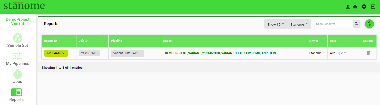
- Click Report ID to access intermediate files from a few important steps in the pipeline.
- Click the PREFIX_ANR.HTML to access the final downloadable report. Default: NO REPORT AVAILABLE.
Reports are generated dynamically based on the analysis type and each report is divided into sections based on the tools used in the pipeline. The first two sections are generated for all the jobs to provide the job overview: analysis summary and sample quality.
- Analysis Summary:
This section consolidates the information related to the job: project, samples, and the experiment in four sub-sections:
-
-
- Project Details: This shows the information provided during the project creation and the pipeline details.
- Run Summary: Displays the job status, runtimes, and the files used for the analysis: reference, annotation or metadata files, and the samples.
- Tools: A brief summary of the tools, versions, descriptions, and citations is shown.
- Commands: A complete list of the commands used in the pipeline.
-
- Sample Quality:
Details of sample (sequencing) quality are provided in this section. It has two sub-sections:
-
-
- Metrics Table: This shows the sequence quality details of each sample in a tabular format.
- Sample Quality Plot: The average quality scores (Phred scale) of all the reads in a sample are displayed in a 96-Well plate format, each circle representing a sample. The higher the score, the better, and scores above 30 are generally considered good for the majority of the applications. Average scores are calculated using all the reads in a sample with the FastQC tool. The 96-Well plate format helps to visualize the low-quality samples, plate effects, and pooling errors easily.
-
The remaining sections are dynamically generated based on the pipeline type and the tools used. Two sample reports are provided below to understand the features of each report.
Variant Report
Variant calling pipelines contains two exclusive sections.
Mapping
This section provides details of the abundance/mapping statistics. This section also has three sub-sections:This
-
-
- Data Table: This (Fig. 1) shows several alignment statistics such as the number of total processed reads, the number of mapped or multi-mapped reads, and the uniquely mapped reads.
- Sample Coverage: Allows users to explore the alignment quality through a series of plots. Sample depth of coverage in total read counts. Sample depth of coverage in percentages. On-target mapping quality in a 96-well plate format
- Read Lengths: Histograms and 96-well plate plots show the read length distributions for mapped and unmapped reads.
- Genome Browser: Aligned reads against the reference genome can be viewed for each sample. The genome browser is interactive and allows exploratory analysis.
-

Variant Calling
This section provides details of the abundance/mapping statistics. This section also has three sub-sections:
-
-
-
- Call Rate Summary: Provides a summary of the genotype calls.
- Target Call Rates: Genotype calling metrics for the top 100 targets are shown in the table format. The complete list can be downloaded from the Reports section. The position field is cross-linked to the Variant Browser. This section also shows:
- Genotype call distribution
- Genotype Heatmap
- Sample Call Rates: Histograms and 96-well plate plots show the call rate distributions from all the samples.
- Genotypes: Shows table of genotypes obtained for each marker across all the samples
- Variant Browser: Sequencing reads support for each variant can be viewed for each sample (Fig. 2). The genome browser is interactive and allows exploratory analysis.
-
-

Transcript Report
This report contains three exclusive sections.
Mapping (Salmon/Kallisto):
This section provides details of the abundance/mapping statistics. This section also has two sub-sections:
-
-
- Data Table: This shows several quasi-alignment statistics such as the number of total processed reads, the number of mapped or multi-mapped reads, and the uniquely mapped reads.
- Plots: Show the sample depth of coverage plots ( mapped and unmapped reads) in raw numbers and percentages.
-
Differential Expression (DE):
Details of the differential expression analysis are dynamically displayed for the pipelines which contain the DE step. This has the following four sub-sections:
-
-
- Data Table: Top 200 most significant Differentially Expressed Genes (DEGs) are listed in tabular format. The table also provides fold change values, confidence levels, and various other parameters. The tool and its various parameters that were used for identifying the DEGs are described briefly below the table. All the important parameters are also described.
- Heatmap: The heatmap (Fig. 1) of the top 200 DEGs. Heatmap visualizes the comparison of DEGs expression across samples and within the sample. A brief description below the map enables users to understand and interpret heatmaps. The red color rectangle in the heatmap indicates the upregulation of a gene and the blue color indicates downregulation.
- PCA & Volcano Plots: A PCA plot enables users to visualize the variability in the replicates of the two experimental conditions compared. All replicates of a condition are depicted with the same color. Grouping of samples indicates if replicates are similar among the same condition versus between the conditions.
- The volcano plot shows significantly differentially expressed genes. It is a scatter plot between log fold change of expression among different biological conditions and the significance of the change determined from the p-value. Volcano plots enable visual inspection of expression change across all the genes.
- Density: Shows normalization plots of samples normalized to overcome bias due to Read size and mRNA content.
-

Annotation (FGSEA):
Describes Pathway analysis for DEGs (Fig.2). The top 100 enriched pathways are shown in the table along with their p-value and the total number of DEGs belonging to the pathway. This section also shows a bubble plot of the enriched pathways wherein the location of the bubble is determined from %DE genes in the enriched pathway to the total number of genes in the pathway.

Jobs
Completed or unfinished pipeline runs are listed in the jobs table on the Jobs window (Fig. 1).

- Click on the jobID to access job details.
- Overview tab lists details of Pipeline run i.e. Job ID, pipeline name and sample set, start and end time of execution, and status.
- Sample Deep-dive (Fig. 2) lists all the sample names.
- Click one sample to check the status or log files for that sample.
- Click the icon on the upper right corner of the jobs details window, to delete the job.
- Stanome generates a consolidated report for each job. The report can be accessed directly by clicking the ReportID on the job details page or through the Reports section from the left-hand menu.
